
PCR and the Binary Communication Channel
PCR and the Binary Communication Channel

*Post too long for email - so you may need to open it in your browser or app
Today, I want to talk about medical testing and why mass testing of asymptomatic individuals is, mathematically speaking, stark raving bonkers. This is something that has been covered in lots of places, but I want to use something called a binary communication channel (BCC) to help us understand what’s going on.
You go to the docs and the doc performs a test that he tells you is “99% accurate”. Sure enough, you get the dreaded result; positive. You’ve almost certainly got the disease, right?
Most people would think this is a no-brainer. Duh, the test is 99% accurate you plank. Of course I’ve got the disease. When someone tells you that this is not so, you might look at them like they’re one of those weird anti-vaxxers, or something like that.
I can’t really blame anyone for thinking like this, because the probability reasoning behind it is not all that easy for the average person (who hasn’t done a course in probability & stats) to understand. It’s one of those seemingly counter-intuitive things that probability often throws at us.
The problem here is that there are two things that are subject to uncertainty, not one. Most people are kind of OK when there’s one thing varying, like a dice roll, for example. They can figure out that their chance of getting an even number when rolling a dice is 1/2, and other things like this.
But when you’ve got two things subject to some uncertainty, and those two things are dependent on one another, then it’s much less easy to figure out the odds.
In medical testing we have these two uncertain things
The uncertainty in the test itself
The uncertainty about whether we have the disease
It’s clear that these things are not wholly independent of one another.
So we have two “variables” here; the test result T, and the disease D. Each of these variables has two possible values; 1 or 0.
T = 1 means the test result is positive, T = 0 means the test result is negative
D = 1 means you have the disease, D = 0 means you do not have the disease
When you get T = 1 at the docs with a 99% accurate test (more on what this means, precisely, in a bit) it’s very tempting to reason that this means you have the disease with a 99% probability. This is the “intuitive” result most people assume. But it’s wrong.
What I’m going to do is to “map” this onto a binary communication channel. This seems a bit crazy at first sight. Why is this fool making things even more complicated? But bear with me, because I think that for some (and I hope all) of you it makes it much easier to see what’s going on with medical testing.
There’s a bit of work to do, but I believe it pays off because this kind of “mapping” onto a BCC is useful for all sorts of other similar probability situations where we have 2 binary variables.
The Binary Communication Channel (BCC)
We live in a digital world and so I’m going to assume that most of you understand that this means things are working by processing bits of data. Everything is all done (at least in principle) by sending, receiving, and processing sequences of 1’s and 0’s. We call these sequences strings of binary digits (bits).
Let’s suppose Alice wants to send a message, in English, to Bob. Our channel can send 1’s and 0’s and so she’s going to have to code her message into binary. One way she could do this is to realize that there are 26 letters in the alphabet and some associated necessary symbols like spaces, full stops, and the like. So, she could use strings that are 5 bits long to do this. She might write
a : 00000
b : 00001
c : 00010
d : 00011
e : 00100
and so on. She could send 32 different symbols this way1. It’s not a particularly efficient way of coding her message, but it gets the job done.
With this coding, the word “bad” gets transmitted as 00001 00000 00011, for example.
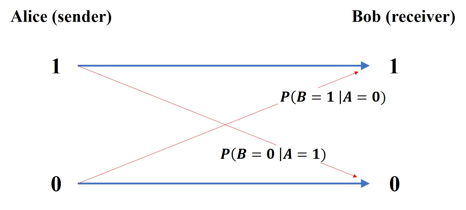
The BCC, schematically, looks like this :

But what are those “cross pieces” in red? They represent errors on the channel. Alice sends a 1, but Bob receives a 0, for example. The usual way to think about this is that there’s some “noise” on the channel that can corrupt the original message a bit.
OK - that looks all reasonably sensible, but where does probability come into all of this?
The thing is that although at any given time Alice is going to be sending a specific message, she could send any message. So if we’re going to understand the properties of the channel we have to treat Alice’s message with the tools of uncertainty.
Let’s face it, if Bob was certain of the message Alice was going to send, what would be the point of the channel in the first place? Put in another way; Alice knows what message she’s sending, but Bob doesn’t.
So, for each timeslot, there’s going to be (from Bob’s perspective) a probability that Alice has selected a 1 or a 0. Similarly, there’s going to be a probability that Bob has received a 1 or a 0.
The job of the receiver is to try to figure out (infer) what message was actually sent from the message he has received.
So, before any message has been received there’s going to be a probability that Alice selects a 1 or a 0. This is going to depend on the set of all possible messages and the way that the message has been coded2.
This is an a priori probability and we’ll label it as P(A) when we’re talking in general about it. There are two probabilities here :
P(A = 1) and P(A = 0)
being the probability that Alice will select a 1 or a 0, respectively. And we’re going to use P(B) when we’re talking about the probability of the bit of the received message.
Errors on the Channel
Much of the difficulty with probability is more of a ‘word’ kind of issue. How you word things is critical, and there’s much confusion to be had if you word things clumsily (as I often do - it takes me a while sometimes to get my head into the ‘right’ word space when doing these probability problems).
So what’s a good way to think about these probabilities P(A) and P(B)?
P(A) : put yourself in Bob’s shoes. He doesn’t know what message Alice is going to send. He does know what coding she’s using and what the set of possible messages looks like. So this is Bob’s assessment of the statistics of what might be sent before any particular message is received.
P(B) : Bob’s received a message containing a million bits. He can work out the number of 1’s and the number 0’s he’s got and so can work out what the probability of getting a 1 is if he selected one of those received million bits at random, for example. P(B) is just this kind of probability.
So these probabilities are a kind of ‘general’ probability - how things stand before we start looking at specifics.
The thing is, is that Alice sends a specific message. Bob doesn’t know what that is, but he hopes he can disentangle it from the bits he actually received.
So what he needs to know is the probability that he receives a 1 given that Alice sent a 1, for example.
Few things in life are perfect and the same goes for communication channels; sometimes they’re going to mess things up. Bob is going to (sometimes) receive a 0 when Alice actually sent a 1 (and vice versa) - and these are errors on the channel.
At this point I probably should mention where we’re heading here. In the context of medical testing an “error” on the channel is going to be when we’ve received a positive test but don’t actually have the disease. The disease status is going to be the “sent” message and the test result will be the “received” message.
How do we characterize errors?
What we do is to use what are called conditional probabilities. We want to know what the probability of receiving a 1 is conditional upon a 0 having been sent (an error). We usually shorten this by using the word “given”.
So we want to know the probability that a 1 has been received given that a 0 was transmitted. That’s a lot of verbiage and so we shorten things up a bit more by using notation
P(B = 1 | A = 0) : means the probability that a 1 was received (B = 1) given that a 0 was sent (A = 0). The vertical line stands for “given”.
So now we can put a bit of flesh on our error bones and label our binary channel schematic like this :
Bob wants to know what message was sent; he needs to infer that from the data he has received. In order to be able do that he needs to know what P(A|B) is, which is the general shorthand for the 4 probabilities :
P(A = 1 | B = 1)
P(A = 0 | B = 0)
P(A = 1 | B = 0) —— this represents an error
P(A = 0 | B = 1) —— this represents an error
But what we have are P(A), P(B) and the error probabilities that characterize the channel which are given by P(B|A).
Note the switch here : what we have are P(B|A) but what we need to be able to figure out the sent message are the probabilities P(A|B).
Error perspective : P(B|A) - probability that a particular B is received, given a particular A was sent
Decoding perspective : P(A|B) - probability that a particular A was sent, given a particular B was received
Note the very different “question” that is being asked by the two different probabilities; P(A|B) and P(B|A) represent different probability questions. That switch of A and B is really important.
Bloody Hell, My Brain’s Melted (and this time it’s not climate change)
I’m sorry. I know for some of you this will (if you even get this far) have been a kind of torture.
But let’s see if we can’t drop in a bit of motivation at this point.
What does all this mean in the context of medical testing?
A medical test is characterized by errors - they’re the forward probabilities in our BCC.
So, we characterize these things by the probability that a test comes up positive given the disease is present (this is called the sensitivity of the test) and we also use the probability that the test comes up negative given the disease is not present (this is called the specificity of the test).
But what the patient is interested in is the backwards probability. He wants to “decode” the test result. What he wants to know is the probability that he has the disease given the test was positive.
It’s that switch again.
The things that characterize the test are like the channel error properties (from Alice to Bob) - the thing the patient wants is, like Bob, the ability to determine what disease “message” was sent given the “test” message that has been received. So we have to go backwards (from Bob’s received message to Alice’s sent message - it’s an inference, or decoding, process).
In medical testing terms, then, we have the probabilities (and we’re back to variables T and D for test result and disease, respectively).
P(T = 1 | D = 1) : the sensitivity of the test. For a perfect test (or ‘channel’) this is just 1. If this is 0.99 (our 99% ‘accurate’ test) then it implies some error exists.
P(T = 0 | D = 0) : the specificity of the test. For a perfect test (or ‘channel’) this is just 1. If this is 0.99 then it means that 1% of our tests give the result 1 when the disease is not present. This is the, per test, false positive rate.
P(D = 1 | T = 1) : this is the thing that our patient (let’s also call him Bob) is interested in. Bob wants to know whether he actually has the disease given that the test result is positive. He wants to figure out what the actual message that was ‘sent’ is.
The Math Bit (you can skip if you want)
So we have these different probabilities that we use to answer different probability questions, but what’s the relationship between them?
I’m doing all of this as I write, with the attitude of “bugger Google”, and so I hope I get this right.
The first thing we note is Bayes’ Theorem which comes from the relationship between the joint, conditional and marginal probabilities :
from which we get
What our patient Bob is interested in is a specific instance of this general result. He wants to know P(D = 1 | T = 1) so let’s put those things into our general expression.
You will notice that we’ve got P(T = 1 | D = 1) on the top on the RHS there - but this is just the test sensitivity. So let’s call this quantity S.
We’ve also got P(D = 1) which is just the probability that if we pick someone from the population at random they have the disease. This is what gets called the prevalence. Here we run into one of the perennial embuggerations with maths. We’ve already got P in use for probability, so what symbol should we give this? Let’s go all a bit Greek and give this the symbol pi.
I also don’t want to keep having to write out P(T = 1 | D = 1) all the time. This is the thing we’re interested in, the question we really want answered, and so let’s just call it Q. This helps the ‘eye’ when looking at algebra, too.
At this stage, then, we have :
Now we need to work a bit to give us an alternative expression for P(T = 1). What we’d like to be able to do is to write our Q in terms of other things we know; the prevalence, the sensitivity, and the specificity. Damn. We’ve already got S in use - so we’re going to need another trip to Athens to pick up a sigma for our specificity.
We have another chat with the good Reverend Bayes and write
You can see how difficult it is to perceive any kind of algebraic ‘pattern’ in expressions like these. To the ‘eye’ it just looks like a bit of a mess. But here’s where the magic of probability comes in. When we sum probabilities over all possibilities we get 1. This is the rule of “something happens”. If we toss a coin then we’re going to get some result. The probability of something happening is 1. So adding up the probability of head and the probability of tail is going to be 1.
The P(D = 0) term can just be written as 1 - P(D = 1), for example, but that’s just 1 minus pi in our notation. The P(T = 1 | D = 0) term is just 1 minus the specificity and the P(D = 0 | T = 1) term is just 1 - Q. So we have :
We plonk this back into our previous expression and get ready to do some faffing about with the algebra, and we eventually end up with the result
So our Q, the thing we’re interested in, the thing that tells us how likely we are to have the disease when we get a positive result, is not simply related to the “accuracy” (the sensitivity) of the test. It involves the specificity and the prevalence too.
There are probably easier ways to derive this relationship, and probably better ways to bring out the ‘meaning’ of what’s going on (rather than just treating it as an exercise in algebraic faffing), but let’s see what it might mean.
One of the things we do when trying to figure out what a mathematical expression means is to look at the ‘limits’. This has a technical meaning, but essentially what we’re trying to do is to see how the expression behaves when a variable ‘approaches’ a particular value.
In this case I want to know what my Q “looks like” as we ramp the prevalence down towards zero. In other words, there’s a disease knocking about but very few people actually have it.
As we turn the prevalence down (as it approaches zero) then the value of Q also approaches zero.
Let’s draw a graph. I’m going to assume a pretty decent test with pi = 0.99 (the sensitivity) and sigma = 0.95 (the specificity)
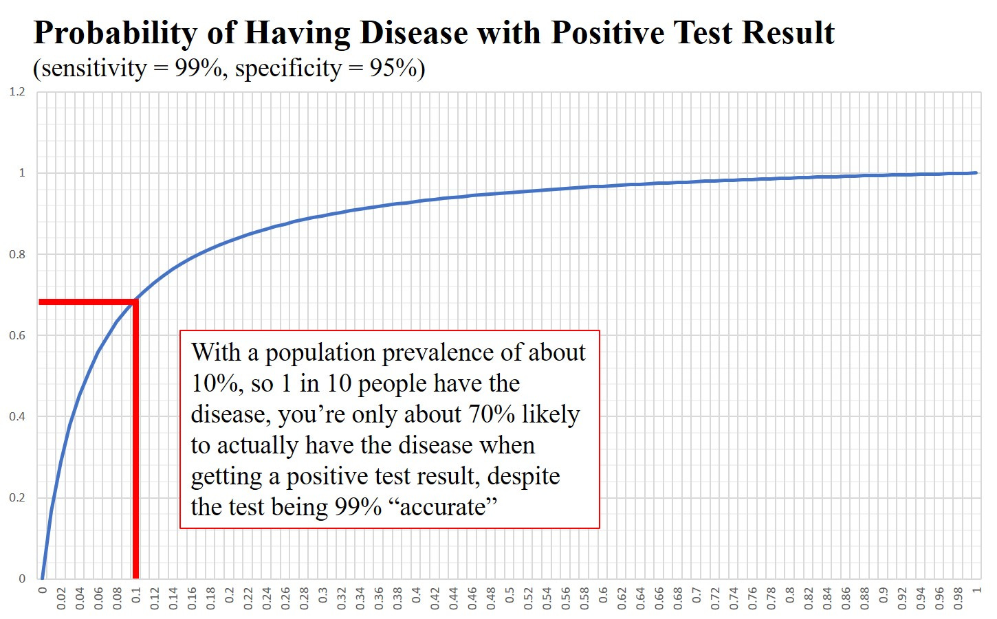
Recall that for covid, prevalence levels, even during one of those ‘waves’, were in the region of 1 in 50. With these parameters (99% sensitivity and 95% specificity) a prevalence of 1 in 50 gives you about a 30% likelihood of actually having the disease when testing positive.
What this means is that about 70% of the people who receive a positive test do not have the disease at all when we have a prevalence of 1 in 50. This is despite the existence of a pretty good “test” for the disease.
How Can We Understand This?
So, we have this seeming paradox; we have a pretty decent test, but 70% of the time it’s wrong when used as a diagnosis for the presence of a disease.
Back to our communication channel.
What does a low prevalence mean in terms of our BCC?
This would be when Alice has chosen a kind of sparse coding. Most of the time she is sending the symbol 0. The channel itself has a pretty low error rate.
If Alice is sending, on average, one 1 for every 50 bits transmitted and the channel has a low(ish) error rate so that 1 —> 0 occurs with probability 1% and 0 —> 1 occurs with probability 5% then about 70% of the 1’s that Bob receives are coming from errors on the channel and not from Alice’s actual message.
In other words if Bob receives a 1 then it is more likely to have come from an error than from the transmitted message.
This is happening because of the difference between the expected incidence of 1’s in one of Alice’s messages (she’s using sparse coding and so we typically expect to see just one 1 for every fifty 0’s, roughly) and the actual incidence of 1’s received (about 5% of the transmitted 0’s will end up as a 1).
You may disagree with me, but I think mapping medical testing onto a BCC makes it much clearer as to what’s happening. It’s kind of obvious when it’s cast in terms of a communication channel.
The downside is that we’ve had to do a bit of work in learning what BCC’s are in the first place.
Once you’ve got your head round this kind of mapping, it can be used for other instances where we have 2 binary random variables. The results sometimes become easier to understand in terms of a communication between Alice and Bob where Bob’s job is to disentangle the actual message of Alice from the data he has received.
Doctors know all about this ‘prevalence problem’. It’s why mass testing of asymptomatic individuals is not recommended. A doctor will (or should) only test people with symptoms. What this does is to, effectively, increase the prevalence. You take a whole population and only look at those with symptoms. In this new, selected, sub-population you’ll have a much higher prevalence and your positive test result will be more likely to be correct.
This is (yet another) of the scientific principles we ditched during covid. Everyone, including those in the medical profession who ought to have known better, went absolutely test crazy. Stuff got shoved up our noses, and in China I think they even shoved things up people’s arses, with gay abandon.
What a waste of bloody time and money it all was - but you have to have some sciency sounding stuff to make people afraid enough.
There are 2 possibilities for the first bit, two possibilities for the second, etc and so the number of distinct symbols she can send with strings of 5 bits in length is going to be 2x2x2x2x2 = 32
Alice could, for example, adopt a code based on strings of 32 bits in length. Each alphabet symbol (or punctuation symbol) would then consist of a string that might look like this
b = 0100 0000 0000 0000 0000 0000 0000 0000. The position of the 1 in the 32 bit string indicating the symbol that is being transmitted. This way of coding would result in a kind of sparse coding where the probability of a zero being transmitted is much higher than that of a 1 for any given timeslot (one 1 is transmitted in every block of 32 bits)
The tests are totally bogus unscientific and not fit for purpose. PCR tests were thoroughly “debunked” by the man who designed them. Lateral flow tests ... don’t make me laugh. I actually sold about a million dollars worth of test kits during the Plandemic so I know a bit about them. The emperors cloths of testing to detect the fake presence of a lie. Still it paid for my 6 rescue cats to eat chicken.... there’s money in invisible cloths.
Well Rudolph you list me in all this but get the gist of it. I agree with IanFenn above. Never trusted the PCR test.